The context for the number field sieve is that we have a composite number N=pq, where p and q are two unknown primes. The key observation behind the number field sieve, as well as the quadratic sieve, is that if we can find x and y such that
x2=y2 mod N,
and x-y is a factor in N. If we are lucky this will be a non trivial factor, giving us the factorization of N.
The difficult part is to find x and y. In the number field sieve this is done by choosing two irreducible polynomials f_1 and f_2, which has a common root m modulo N. In our case f_1 one is a polynomial of degree 5 and f_2=(x-m). Let \alpha_1 and \alpha_2 be roots of f_1 and f_2, respectively, in C. Let Q_N be the ring of rational numbers with denominator coprime to N. The idea is to find a set S of pairs (a,b) of coprime integers such that both \prod_S(a-b\alpha_1) and \prod_S(a-b\alpha_2) are squares in Q_N[\alpha_1] and Q_N[\alpha_2] respectively.
The polynomial we selected was the following.
f(X) = -6247082964584147017624605573745 + 15936731544836237834459094286 X + 2829297479513907345825891 X2 - 1172935345297812805690 X3 - 151784366195895734 X4 + 16464033265680 X5
This polynomial was found using the program gnfsnew written by Peter Montgomery. The information about the polynomial given by the program was the following.
m :=  14551781212637956077810103322;
f := -5441150002907296121437025528667
   +  15959309584940051014641790739 * X^1
   +      2815207694608160076202347 * X^2
            -1175361260911624628634 * X^3
                -151455085530582134 * X^4
   +                 16464033265680 * X^5;
Suggested a/b ratio 4195.478493.  Average = 50.1917
Lead factors:  2^4  3^3  5  7  11  13  17  31.  Cofactor = 14449
GCD(lead coefficient, square of 2nd) = 28


f + (0 X + 51)*(X - m), then X <- X + -4
   size  50.19,  modular   4.61,  net  45.59,  ratio    4190.34, content 1
[16464033265680, -151784366195895734, -1172935345297812805690,
 2829297479513907345825891, 15936731544836237834459094286,
 -6247082964584147017624605573745,
 14551781212637956077810103326,      4190.34, 50.19, 4.61, 1]
We found polynomials with higher score than this after we had
started sieving, but at that time we did not feel like starting
all over again.


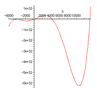
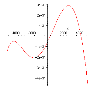
If we plot the polynomial we see that it has three real roots, and a local maximum rather closely below the x-axis.
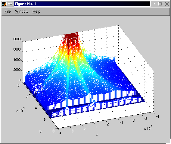
The image above shows the number of relations obtained for different values of the parameters a and b. The graph is basically a histogram. We have divided the a-range into intervals of length 10^8 and the b-range inte intervals of length 10^3. The number of relations found for pairs (a,b) in each bin is then displayed. To make the graph more visible we have cut the peak at 8000.
We observe that there are four clearly marked ridges in the plot. This is also what we would expect from the graphs above. What we are factoring to find relations are basically the norm of the polynomials. For the five degree polynomial this means that we want to factor b^5f(a/b). When this number is small there will be greater chance that the number is smooth, i.e., has small prime factors, and thus gives a relation. The three ridges lying in the positive a-plane thus correspond to the three real roots of the polynomial, and the ridge in the negative a-plane corresponds to the local maximum for f near X=-4000.
As can be seen there are some holes in the sieving area. The explanation for these holes are that we did not use the same a-range in all sieving jobs. Our aim was naturally to search for relations in the area where the densitity of the relations were as high as posible. After having sieved for a while our impression was that the number of relations found for large absolute values of a was small, and we therefore scaled down the a range. Later on, when we realized that the area we first thought would be sufficient was not enough, we started filling in the holes in these flanking areas.